Compositional Visual Retrieval
Fine-Grained Patch-Level Understanding for Compositional Object Modifications
TL;DR: Our Approach in a Nutshell
Our model leverages FILIP (Fine-grained Image-Language Interaction with Patch-level) to understand which image patches correspond to which text tokens, enabling precise localization of object parts. We then introduce a Combiner module that learns to compositionally modify reference images based on textual instructions, generating target image embeddings that match the desired modifications.
The key innovation is our two-stage training approach: first learning fine-grained patch-text alignments through FILIP's token-wise contrastive learning, then training a lightweight MLP-based Combiner to perform vector arithmetic in embedding space for compositional retrieval.
We employ advanced dataset expansion techniques including chain triplets and reverse triplets to create synthetic training data, while using anti-collapse loss functions (InfoNCE + MSE + Consistency) to maintain discriminative embeddings during the compositional mapping process.
Q5 Overview and Dataset Understanding
In the RAYAN Challenge, Q5 was the first final-stage question on the leaderboard. It tested our model's ability to handle basic compositional retrieval tasks from the training dataset. The key was to understand the dataset deeply:
- Simple objects: All images show simple objects on a plain gray background. However, they mentioned that the testing images might be different, so we needed to consider the distribution shift
- No overlaps: Objects are completely separate from each other
- Compositional queries: Text modifies objects like "remove motor and add microwave"
- Fine-grained understanding: Model must spot individual parts and change them mentally
Our Approach and Methodology
We built on OpenCLIP (ViT-B/16 backbone) as our base, since it's allowed if fine-tuned. The pipeline has two main steps:
Stage 1: FILIP Pretraining
- Convert CLIP to patch-aware model
- Learn fine-grained image-text alignments
- Use keyword-based hard negative mining
Stage 2: Compositional Retrieval
- Train Combiner module for modification tasks
- Generate target embeddings from reference + text
- Use triplet training with anti-collapse losses
Dataset Preparation: Offline Captioning with Quantized VLM
Challenge: No Image-Text Pairs Available
We started with 50K training images but no captions. Solution: Generate them using a quantized Llama-3B model locally.
| Step | Method | Purpose |
|---|---|---|
| 1. Model | Llama-3B (4-bit quantized) | Create text-image pairs for FILIP training, captioning all given data for FILIP model training |
| 2. Prompt | "Describe this image in detail, listing objects" | Generate structured object lists |
| 3. Augmentation | Paraphrase variations | Increase text diversity |
| 4. Output | 50K image-caption pairs + 3K modification texts | Rich training data for pretraining and model fine tuning |
📝 Captioning Challenges & Serendipitous Gains
Challenge: Lack of Structured Position Information
Ideally, we wanted structured outputs like {"objects": [{"name": "hat", "position": "top-left"}, ...]} to explicitly teach spatial awareness. However, the quantized Llama-3B model lacked reliable structured output capabilities, and forcing JSON formatting resulted in frequent parsing errors and hallucinations.
Our Solution: We simplified the prompt to free-form descriptions: "Describe this image in detail, listing objects you see."
✅ Unexpected Benefit: Natural Data Augmentation
What Happened: The model sometimes spontaneously generated richer descriptions than requested!
Basic Output:
"hat, chair, train"
Enhanced Output:
"blue cap on the top left, wooden chair in the center, toy train at the bottom"
Why This Helped: This variability acted as implicit data augmentation for handling distribution shifts during evaluation. Some captions were minimal (object names only), while others included colors, positions, and attributes. This diversity helped the model generalize better to different test query styles.
- Robustness: Model learns to match both "hat" and "blue cap on top left" to the same patch
- Distribution Shift Mitigation: Test queries might use different vocabulary or detail levels
- Free Augmentation: No manual effort required—model naturally varied output complexity
🔄 Text Modification Augmentation
Beyond image captions, we also augmented the modification texts to handle linguistic diversity in the dataset.
Dataset Observation: Training data showed varied phrasing patterns:
- Majority pattern (~85%): "remove item X and add item Y"
- Variations (~15%): "get rid of item X and add item Y to this", "add item Y for this and get rid of item Z"
Augmentation Strategy: We prompted Llama-3B to paraphrase modification texts:
Outputs:
- "include a chair and get rid of the motor"
- "put in a chair and take out motor"
- "add a chair to this, remove the motor"
Result: Generated ~3K augmented modification texts, which were crucial for Stage 2 (Combiner training) to make the text encoder more robust to paraphrasing and linguistic variations.
FILIP Mechanism: Fine-Grained Patch-Level Understanding
FILIP Architecture: Dual Encoders with Late Interaction
Image Encoder
- ViT-B/16 processes image into 196 patches
- Each patch: 768-dim feature vector
V ∈ ℝ^{196×768}
Text Encoder
- Tokenizes caption into ~77 tokens
- Each token: 768-dim embedding
T ∈ ℝ^{77×768}
Core Innovation: Token-Wise Max Similarity
FILIP Architecture: Bidirectional Late Interaction
Unlike standard CLIP which only compares global [CLS] tokens, FILIP performs fine-grained matching between all text tokens and all image patches. This enables precise localization of which words correspond to which image regions.
Step 1: Compute Token-Patch Similarity Matrix
For each text token \(i\) and image patch \(j\), compute dot product similarity:
where \(\mathbf{T}_i \in \mathbb{R}^{768}\) is the i-th text token, \(\mathbf{V}_j \in \mathbb{R}^{768}\) is the j-th image patch
This creates a similarity matrix \(S \in \mathbb{R}^{N_t \times N_v}\) where \(N_t = 77\) text tokens and \(N_v = 196\) image patches.
Step 2: Max Pooling - Find Best Matching Patch per Token
Why Max? Each text token should match the most relevant image patch. For example, the word "motor" should strongly align with engine patches, not background regions.
For each text token, find its highest similarity across all image patches
Step 3: Average Pooling - Aggregate to Global Score
After finding the best match for each token, average across all tokens to get the global image-text similarity:
Average of max similarities across all text tokens
Step 4: Bidirectional Matching (Image-to-Text)
To ensure symmetry, we also compute the reverse direction: for each image patch, find its best matching text token:
For each patch, find best token, then average across all patches
Final Similarity Score (Symmetric)
The final FILIP similarity combines both directions:
Symmetric matching ensures both text and image contribute equally
🔧 PyTorch Implementation with Einops
import torch
import torch.nn.functional as F
from einops import einsum, reduce

def filip_similarity(image_features, text_features, temperature=0.07):
    """
    Compute FILIP similarity with bidirectional token-wise matching

    Args:
        image_features: [batch_size, num_patches, dim] e.g. [B, 196, 768]
        text_features:  [batch_size, num_tokens, dim] e.g. [B, 77, 768]
        temperature: softmax temperature for contrastive learning

    Returns:
        similarity_matrix: [batch_size, batch_size] global similarities
    """
    # Normalize features
    image_features = F.normalize(image_features, dim=-1)  # [B, 196, 768]
    text_features = F.normalize(text_features, dim=-1)    # [B, 77, 768]

    # Compute token-patch similarity matrix using einops
    # Each text token from sample i vs all patches from sample j
    similarity = einsum(
        text_features, image_features,
        'b_t n_t d, b_v n_v d -> b_t b_v n_t n_v'
    )  # [B, B, 77, 196]

    # Text-to-Image: Max pooling over patches, then average over tokens
    t2i_max = reduce(similarity, 'b_t b_v n_t n_v -> b_t b_v n_t', 'max')  # [B, B, 77]
    t2i_score = reduce(t2i_max, 'b_t b_v n_t -> b_t b_v', 'mean')  # [B, B]

    # Image-to-Text: Max pooling over tokens, then average over patches
    i2t_max = reduce(similarity, 'b_t b_v n_t n_v -> b_t b_v n_v', 'max')  # [B, B, 196]
    i2t_score = reduce(i2t_max, 'b_t b_v n_v -> b_t b_v', 'mean')  # [B, B]

    # Symmetric averaging
    final_similarity = (t2i_score + i2t_score) / 2  # [B, B]

    # Apply temperature scaling
    logits = final_similarity / temperature

    return logits
🎯 Key Insight: The two-stage pooling is crucial: (1) Max pooling over patches captures the strongest alignment for each token (e.g., "motor" → engine patch), producing a [77×1] vector. (2) Mean pooling over tokens aggregates these max similarities into a single scalar score. The bidirectional design (text-to-image + image-to-text) ensures both rare words and small patches contribute fairly to the final similarity.
FILIP Architecture: Late Interaction for Fine-Grained Alignment
224×224
Encoder
train center,
hat bottom"
Encoder
🎯 Late Interaction: Token-Patch Matching
🔍 How it works: The similarity matrix \(S \in \mathbb{R}^{77 \times 196}\) shows alignment between each text token (rows) and each image patch (columns).
Step 1 - Max Pooling: For each text token (row), we find the maximum similarity across all 196 image patches (columns). This gives us a vector of shape [77×1], where each value represents the best patch match for that token. Example: "chair" token → highest similarity with chair patches (green cells).
Step 2 - Mean Pooling: We average all 77 max similarities across text tokens to get a single scalar score. This aggregates information from all words to produce the final text-to-image similarity score. The same process runs in reverse (image-to-text) for bidirectional matching.
FILIP Training Dataset: Strategic Data Mix & Augmentation
📊 Data Mix Strategy
Training Ratio for FILIP Pretraining
To train FILIP effectively for compositional retrieval, we carefully balanced general image-text alignment (captions) with task-specific compositional understanding (modification queries).
Generated Captions (80%)
Generated by Llama-3B, describing objects in each image. These teach general image-text alignment.
Example Captions:
"cat, car, bus""wooden chair top-left, toy train center, blue hat bottom""microwave, lamp, bicycle""red motor on top, green chair middle, yellow hat below"
Purpose: Maintain broad visual-linguistic understanding and prevent overfitting to only compositional modifications.
Modification Queries (20%)
Task-specific queries about adding/removing objects. Critical for compositional reasoning.
Example Queries:
"remove the bike and add the car""add chair, remove lamp""get rid of motor and place microwave"
Purpose: Teach model to parse compositional instructions and attend to specific object patches.
🎯 Why This 80-20 Split?
Too Much Caption (95%+):
Model learns general alignment but fails at compositional tasks. Doesn't understand "add/remove" semantics.
Too Much Query (50%+):
Overfits to specific modifications. Poor generalization to novel object combinations and test distribution shifts.
80-20 balance: Best of both worlds—maintains general understanding while learning task-specific compositional reasoning.
🛡️ LoRA: Preventing Catastrophic Forgetting Under Distribution Shift
The Distribution Shift Problem
The RAYAN challenge explicitly warned about potential "distribution shifts" between training and test data. Fine-tuning the entire OpenCLIP model risked catastrophic forgetting—losing general visual knowledge to overfit on the specific training distribution.
Potential Distribution Shifts:
- Novel object combinations not seen in training
- Different linguistic phrasings of modifications
- Variations in image quality, lighting, or backgrounds
- Objects in unusual positions or orientations
Why LoRA (Low-Rank Adaptation)?
❌ Full Fine-Tuning Problems
- Updates all 149M parameters
- Catastrophic forgetting of general knowledge
- Overfits to training distribution
- Poor generalization to shifts
✅ LoRA (rank=32) Benefits
- Updates only ~0.1% of parameters
- Preserves pretrained knowledge
- Adapts to task-specific patterns
- Better generalization to unseen data
How LoRA Works: Low-Rank Parameter Updates
Instead of updating weight matrix \(W \in \mathbb{R}^{d \times d}\) directly, LoRA adds a low-rank decomposition:
where \(B \in \mathbb{R}^{d \times r}\), \(A \in \mathbb{R}^{r \times d}\), and \(r \ll d\) (rank=32 ≪ 768)
Full Fine-Tune
768 × 768
~590K params/layer
LoRA (r=32)
768×32 + 32×768
~49K params/layer
Reduction
92%
fewer parameters
🎯 Result: LoRA allowed us to adapt FILIP to the specific task (compositional retrieval) while preserving OpenCLIP's broad visual understanding. This proved crucial when test queries used novel object combinations or unexpected phrasings—the model fell back on its pretrained knowledge instead of failing completely.
| Training Aspect | Configuration | Reasoning |
|---|---|---|
| Backbone | OpenCLIP ViT-B/16 | Strong pre-trained features |
| Fine-tuning | LoRA (rank=32) | Preserves knowledge, prevents catastrophic forgetting |
| Batch Size | 16 | Memory constraints |
| Epochs | 10 | Convergence without overfitting |
| Data Mix | 80% captions + 20% queries | Balance general alignment with compositional reasoning |
| Augmentation | Keyword swap + Paraphrasing | Doubles compositional data, linguistic robustness |
| Training Time | 36 hours | Single RTX 3090 |
Hard Negative Mining: An Attempted Enhancement
After successfully pretraining FILIP, we hypothesized that adding hard negative mining could further improve the model's discriminative ability. This section documents our implementation and the surprising lack of improvement—an honest account of an experiment that didn't work as expected.
What is Hard Negative Mining?
Concept: Learning from "Tricky" Wrong Examples
In contrastive learning, hard negatives are negative samples that are semantically similar to the positive sample but not quite correct. These are "tricky" examples that force the model to learn fine-grained differences.
✅ Easy Negatives (Random Sampling)
Query:
"chair, train, hat"
Easy Negative:
"dog, tree, bicycle"
Problem: Too easy! Model quickly learns these are different. No fine-grained learning.
🎯 Hard Negatives (Targeted Sampling)
Query:
"chair, train, hat"
Hard Negative:
"chair, train, lamp"
↑ 2 objects match, 1 differs
Benefit: Tricky! Forces model to distinguish subtle differences (hat vs lamp).
🎯 Goal: By training on hard negatives, the model learns to pay attention to fine details and object-level differences, not just overall image similarity. This should improve precision in compositional retrieval tasks.
Our Implementation: Keyword-Based Hard Negative Selection
Step 1: Keyword Extraction from Comma-Separated Captions
Since our generated captions were already in comma-separated format (e.g., "chair, train, hat"), extracting keywords was straightforward—simply split by commas and clean whitespace.
🔧 Python Implementation
import re
from collections import defaultdict

def extract_keywords(caption):
    """
    Extract object keywords from comma-separated captions
    """
    # Split by comma and clean
    keywords = [k.strip().lower() for k in caption.split(',')]

    # Remove articles and common words
    stop_words = {'a', 'an', 'the', 'on', 'in', 'at', 'of'}
    keywords = [' '.join([w for w in k.split() if w not in stop_words])
                for k in keywords]

    return set(keywords)

# Example usage
caption1 = "wooden chair, toy train center, blue hat"
caption2 = "red car, wooden chair, lamp"
caption3 = "bicycle, motor, hat"

keywords1 = extract_keywords(caption1)  # {'wooden chair', 'toy train center', 'blue hat'}
keywords2 = extract_keywords(caption2)  # {'red car', 'wooden chair', 'lamp'}
keywords3 = extract_keywords(caption3)  # {'bicycle', 'motor', 'hat'}

# Find overlap
overlap_1_2 = len(keywords1 & keywords2)  # 1 ('wooden chair')
overlap_1_3 = len(keywords1 & keywords3)  # 1 ('hat')
Key Insight: The comma-separated format made it trivial to parse objects without needing complex NLP or object detection models.
Step 2: Hard Negative Batch Construction
Strategy: Create batches where each sample has at least one hard negative with exactly 2 matching objects and 1 different object.
Matching Criteria
For each anchor sample with objects {A, B, C}:
- Hard Negative: Must have 2 objects from {A, B, C} + 1 different object D
- Example: Anchor = "chair, train, hat" → Hard Negative = "chair, train, lamp"
- Overlap: |keywords_anchor ∩ keywords_negative| = 2
🔧 Hard Negative Batch Sampler
def create_hard_negative_batch(dataset, batch_size=16):
    """
    Create batches with hard negatives (2 matching objects, 1 different)
    """
    # Index dataset by keywords
    keyword_index = defaultdict(list)
    for idx, (image, caption) in enumerate(dataset):
        keywords = extract_keywords(caption)
        # Store by keyword combinations
        for k in keywords:
            keyword_index[k].append((idx, keywords))

    batches = []
    used_indices = set()

    for idx, (image, caption) in enumerate(dataset):
        if idx in used_indices:
            continue

        anchor_keywords = extract_keywords(caption)
        if len(anchor_keywords) != 3:  # Skip if not exactly 3 objects
            continue

        # Find hard negatives: 2 matching + 1 different
        batch = [(idx, anchor_keywords)]

        for other_idx, other_keywords in dataset:
            if other_idx == idx or other_idx in used_indices:
                continue

            overlap = len(anchor_keywords & other_keywords)

            # Hard negative: exactly 2 objects match
            if overlap == 2:
                batch.append((other_idx, other_keywords))
                used_indices.add(other_idx)

                if len(batch) >= batch_size:
                    break

        if len(batch) >= batch_size // 2:  # At least half filled
            batches.append(batch)
            used_indices.add(idx)

    return batches

# Example batch
# Anchor:   "chair, train, hat"      (positive)
# Hard Neg: "chair, train, lamp"     (2 match: chair, train | 1 diff: lamp vs hat)
# Hard Neg: "chair, motor, hat"      (2 match: chair, hat | 1 diff: motor vs train)
# Hard Neg: "bicycle, train, hat"    (2 match: train, hat | 1 diff: bicycle vs chair)
Visual Example of a Hard Negative Batch
"chair, train, hat"
"chair, train, lamp"
✓ chair ✓ train ✗ lamp
"chair, motor, hat"
✓ chair ✗ motor ✓ hat
"bicycle, train, hat"
✗ bicycle ✓ train ✓ hat
Step 3: Training with Hard Negatives
Training Configuration
| Parameter | Value | Reasoning |
|---|---|---|
| Batch Size | 16 | Same as base FILIP training for consistency |
| Epochs | 1.5 | Short fine-tuning on top of pretrained FILIP |
| Learning Rate | 5e-5 | Lower than pretraining to avoid catastrophic forgetting |
| Hard Negatives per Batch | 8-12 | ~50-75% of batch are hard negatives |
| Loss Function | FILIP InfoNCE (unchanged) | Hard negatives naturally get higher loss |
Hypothesis: By exposing the model to more challenging negatives, we expected 2-3% improvement in Top-1 accuracy, especially on edge cases where objects differ by only one item.
❌ Results: No Meaningful Improvement
Experimental Outcomes
| Model Variant | Top-1 Val (%) | R@5 (%) | R@10 (%) | Notes |
|---|---|---|---|---|
| FILIP (Base) | 85.5 | 87.2 | 93.6 | After pretraining (10 epochs) |
| FILIP + Hard Negatives (1.5 epochs) | 63.8 | 86.8 | 93.2 | -0.7% (slight degradation) |
| FILIP + Hard Negatives (3 epochs) | 63.3 | 86.0 | 92.8 | -1.2% (moderate degradation) |
🔍 Key Observation
Disappointing Result: Despite our hypothesis, hard negative mining provided no meaningful improvement. In fact, training for more epochs (3) slightly degraded performance, suggesting potential overfitting to the hard negative distribution.
🤔 Why Did Hard Negative Mining Fail?
In retrospect, we identified several reasons why this approach didn't improve the model:
1️⃣ Already Hard Enough
FILIP's in-batch negatives (batch size 16) were already challenging. The model was seeing 15 negatives per sample, many of which naturally overlapped in objects. Adding "harder" negatives was redundant.
2️⃣ Coarse Algorithm
Our keyword matching was too simplistic. It only counted exact string matches and ignored semantic similarity (e.g., "chair" vs "seat", "motor" vs "engine"). Many "hard negatives" weren't actually semantically close.
✅ What Would Have Worked Better (In Hindsight)
Smarter Hard Negative Mining Strategies
🎯 Semantic Similarity-Based Mining
Use embedding similarity instead of keyword matching:
- Compute CLIP embeddings for all captions
- Sample negatives with cosine similarity 0.6-0.8 (close but not identical)
- Expected gain: +2-3%
🎯 Soft Margin Loss
Weight negatives by difficulty:
- Hard negatives get higher loss weight
- Easy negatives get lower weight
- Prevents collapse on overly hard negatives
Recommendation: If implementing hard negative mining, invest time in a robust selection algorithm (embedding-based) and use soft weighting. Our simple keyword approach was insufficient for this task.
Interpretability Analysis: Ensuring Right-Region Attention
To confirm "did it learn to look at exact parts?", we use Grad-CAM (Gradient-weighted Class Activation Mapping)—gradients highlight what influences decisions.
🔬 How Grad-CAM Works in Our Pipeline
For a query like "this image contains a bus", we backpropagate from the target embedding through the image encoder to visualize which patches contribute most to the decision.
Grad-CAM Computation Steps
Encode reference image through FILIP
Generate target embedding for query
Gradients flow to patch features
Create heatmap overlay
Mathematical Formulation
\(A^k\): activation maps for patch \(k\), \(\alpha_k\): importance weights from gradients, \(y\): target similarity score
🎯 Key Insight: Gradients weight patch activations by their contribution to the target embedding. High gradient magnitude → patch is important for the query. ReLU removes negative contributions (irrelevant regions).
🎯 Grad-CAM: CLIP vs FILIP Comparison
Heat intensity shows attention strength: Blue = High attention, Red = Low attention, Gray = Medium attention
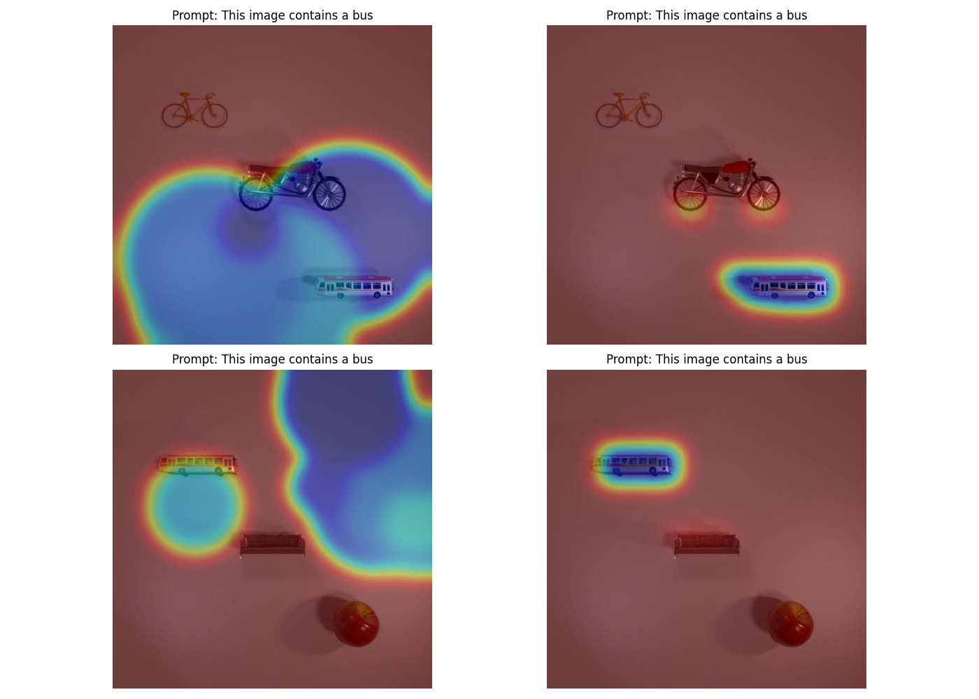
Figure: Grad-CAM attention heatmaps for query "This image contains a bus"
🔍 Key Observations:
- Left (Standard CLIP): Diffuse attention spreads across the entire image with no clear focus. The model treats the image as a holistic "blob" and fails to localize specific objects mentioned in the query.
- Right (FILIP): Concentrated attention forms distinct "halos" around the bus object in multiple scenes. Sharp boundaries clearly delineate the target object from background elements (bicycles, motorcycles, sofas).
- Precision: FILIP's attention peaks align with actual bus regions, demonstrating fine-grained patch-level understanding that CLIP lacks.
📊 Experimental Findings: Pre-FILIP vs Post-FILIP
❌ Pre-FILIP (Standard CLIP)
- Diffuse Attention: Heatmaps smear over the entire image
- No Localization: Cannot distinguish "motor" from "chair" or background
- Global Matching Only: Relies on overall image similarity, not part-level understanding
✅ Post-FILIP (Fine-Grained Model)
- Sharp Focus: Heatmaps concentrate on relevant object patches
- Precise Localization: "Bus" query lights up bus area (blue), rest stays cool (red)
- Patch-Level Understanding: Token-wise max similarity enables fine-grained attention
Stage 2: Compositional Embedding Generation
Challenge: From Understanding to Transformation
After FILIP pretraining, our model could understand which patches belong to which text tokens, but couldn't create new embeddings representing modified images.
Goal: Generate a single vector that matches target images based on reference_image + modification_text.
Combiner Architecture
Combiner Module: Lightweight MLP for Compositional Mapping
The Combiner takes [CLS] tokens from image and text encoders (768-dim each) and outputs a single 768-dim target embedding through learned gated residual fusion.
Complete Architecture Implementation
import torch
import torch.nn as nn
import torch.nn.functional as F

class Combiner(nn.Module):
    """
    Compositional embedding generator with dynamic gated residual fusion

    Architecture:
        1. Project image and text features to higher dimension (1024d)
        2. L2 normalize projections for stable training
        3. Concatenate normalized features
        4. Main path: MLP fusion (2048d hidden → 768d output)
        5. Gate path: Parallel sigmoid gate for adaptive weighting
        6. Final: Gated residual combination of fused + text + image
    """
    def __init__(self, dim=768, proj=1024, hidden=2048):
        super().__init__()

        # Projection layers (expand to higher dimension)
        self.img_proj   = nn.Linear(dim, proj)   # 768 → 1024
        self.text_proj  = nn.Linear(dim, proj)   # 768 → 1024

        # Main fusion MLP
        self.combine    = nn.Linear(proj*2, hidden)  # 2048 → 2048
        self.out        = nn.Linear(hidden, dim)     # 2048 → 768

        # Dynamic gating mechanism (key innovation)
        self.gate = nn.Sequential(
            nn.Linear(proj*2, hidden),  # 2048 → 2048
            nn.ReLU(),
            nn.Dropout(0.5),            # regularization
            nn.Linear(hidden, 1),       # 2048 → 1
            nn.Sigmoid()                # α ∈ [0, 1]
        )

        # Learned temperature for contrastive retrieval
        self.logit_scale = nn.Parameter(torch.ones([]) * 4.605)  # ln(100)

    def forward(self, img_feat, text_feat):
        """
        Args:
            img_feat: [B, 768] reference image CLS tokens
            text_feat: [B, 768] modification text CLS tokens

        Returns:
            final: [B, 768] predicted target embedding (L2 normalized)
        """
        # Step 1: Project and normalize features
        i = F.normalize(self.img_proj(img_feat), dim=-1)   # [B, 1024]
        t = F.normalize(self.text_proj(text_feat), dim=-1) # [B, 1024]

        # Step 2: Concatenate for joint processing
        cat = torch.cat([i, t], dim=-1)  # [B, 2048]

        # Step 3: Compute gating weight (parallel path)
        alpha = self.gate(cat)  # [B, 1] - adaptive weight α ∈ [0, 1]

        # Step 4: MLP fusion (main path)
        fused = self.out(F.gelu(self.combine(cat)))  # [B, 768]

        # Step 5: Gated residual fusion (best performing combination)
        # final = fused + α * text + (1 - α) * image
        final = fused + alpha * text_feat + (1 - alpha) * img_feat

        # Step 6: L2 normalize for cosine similarity retrieval
        final = F.normalize(final, dim=-1)  # [B, 768]

        return final
Mathematical Formulation: Gated Residual Fusion
The core innovation is the gated residual fusion mechanism that adaptively combines three signals:
Parallel Processing:
α = gating weight, f = fused features
Final Gated Residual Combination:
Three-way fusion: learned features + weighted text influence + weighted image preservation
Why Gated Residual Fusion Works Best
Minor Modifications (α ≈ 0.2)
Query: "add small lamp"
Preserves 80% of reference image features, adds 20% text direction
Major Transformations (α ≈ 0.8)
Query: "remove all objects, add car"
Heavy modification: 20% reference, 80% text direction
Key Advantages:
- Adaptive: Gate learns per-query how much to transform (not fixed arithmetic)
- Residual: Direct paths from inputs prevent gradient vanishing
- Stable: L2 normalization at each step maintains unit sphere embeddings
🔧 Combiner Forward Pass Visualization
768d
768d
1024d
1024d
Norm
Norm
2048d
2048→2048
2048→768
Fusion
768d
🎯 How Gating Works: The sigmoid gate (α) decides how much to "move" from reference image toward text direction. For minor changes (α≈0.2), mostly preserves reference. For major changes (α≈0.8), heavily modifies embedding.
🔀 Parallel Gating Path Architecture
The gating mechanism runs in parallel to the main MLP path to dynamically weight the combination
2048→2048
p=0.5
2048→1
Purpose: The gate value α controls the final fusion: final = fused + α·text + (1-α)·img
High α (≈0.8) = major modification, Low α (≈0.2) = minor refinement
Training with Anti-Collapse Losses
Triplet Training: (Reference, Text, Target)
We train with real triplets using three complementary losses to prevent embedding collapse. Each loss serves a specific purpose in maintaining discriminative, well-separated embeddings.
Complete Loss Implementation
def compute_triplet_loss(combiner, ref_feat, text_feat, target_feat, db_features):
    """
    Compute anti-collapse loss for compositional retrieval

    Args:
        ref_feat: [B, 768] reference image CLS tokens
        text_feat: [B, 768] modification text CLS tokens
        target_feat: [B, 768] ground truth target image CLS tokens
        db_features: [N, 768] database of all target embeddings for retrieval

    Returns:
        total_loss: weighted sum of three complementary losses
    """
    # Generate predicted target embedding
    pred = combiner(ref_feat, text_feat)  # [B, 768]

    # ============================================
    # Loss 1: InfoNCE (Contrastive Loss)
    # ============================================
    logits = pred @ db_features.T * combiner.logit_scale.exp()  # [B, N]
    labels = torch.arange(len(pred), device=pred.device)
    loss1 = F.cross_entropy(logits, labels)

    # ============================================
    # Loss 2: MSE (Direct Alignment Loss)
    # ============================================
    loss2 = F.mse_loss(pred, target_feat)

    # ============================================
    # Loss 3: Consistency Loss (Geometry Preservation)
    # ============================================
    dist_pred = torch.cdist(pred, pred)           # [B, B]
    dist_tgt = torch.cdist(target_feat, target_feat)  # [B, B]
    loss3 = F.mse_loss(dist_pred, dist_tgt) * 0.1

    # Combined loss
    total_loss = loss1 + loss2 + loss3

    return total_loss, loss1, loss2, loss3
Loss Component 1: InfoNCE (Contrastive Loss)
Purpose: Pulls predicted embeddings close to correct targets while pushing away from incorrect targets (negatives). This creates discriminative boundaries in embedding space.
Mathematical Formulation
where \(B\) = batch size, \(N\) = database size, \(\tau\) = temperature (learned via logit_scale)
PyTorch Implementation
# Compute similarity scores (logits)
logits = pred @ db_features.T  # [B, N] - cosine similarity
logits = logits * combiner.logit_scale.exp()  # scale by learned temperature

# Ground truth: diagonal elements are positive pairs
labels = torch.arange(B, device=pred.device)  # [0, 1, 2, ..., B-1]

# Cross-entropy treats row i, column i as positive
loss1 = F.cross_entropy(logits, labels)
🎯 Why This Works: For each predicted embedding, InfoNCE maximizes similarity with its correct target (numerator) while minimizing similarity with all other targets in the database (denominator). This prevents mode collapse by forcing the model to maintain distinct embeddings for different compositions.
Loss Component 2: MSE (Direct Alignment Loss)
Purpose: Forces the predicted embedding to exactly match the ground truth target embedding. This provides a strong supervised signal for precise alignment.
Mathematical Formulation
where \(\mathbf{z}_i^\text{pred} \in \mathbb{R}^{768}\) is the predicted embedding, \(\mathbf{z}_i^\text{target} \in \mathbb{R}^{768}\) is the ground truth
PyTorch Implementation
# Direct L2 distance between predicted and target
loss2 = F.mse_loss(pred, target_feat)

# Equivalent to:
# loss2 = torch.mean((pred - target_feat) ** 2)
🎯 Why This Works: While InfoNCE focuses on relative similarities (ranking), MSE provides absolute positioning. This ensures predictions don't just rank correctly but actually land in the right region of embedding space. Without MSE, predictions might correctly distinguish targets but be geometrically far from ground truth.
Loss Component 3: Consistency Loss (Geometry Preservation)
Purpose: Preserves the relative distances between samples in embedding space. If two targets are close in ground truth space, their predictions should also be close. This maintains the geometric structure of the embedding manifold.
Mathematical Formulation
where \(D_{ij}^\text{pred} = \|\mathbf{z}_i^\text{pred} - \mathbf{z}_j^\text{pred}\|_2\) and \(D_{ij}^\text{target} = \|\mathbf{z}_i^\text{target} - \mathbf{z}_j^\text{target}\|_2\)
PyTorch Implementation
# Compute pairwise distance matrices
dist_pred = torch.cdist(pred, pred)              # [B, B]
dist_tgt = torch.cdist(target_feat, target_feat) # [B, B]

# Minimize difference between distance structures
loss3 = F.mse_loss(dist_pred, dist_tgt) * 0.1   # weight = 0.1

# This ensures:
# If target A and B are close → predictions A' and B' should be close
# If target A and C are far → predictions A' and C' should be far
🎯 Why This Works: Consistency loss prevents the model from creating "shortcuts" where all predictions cluster together (mode collapse). By forcing the predicted distance matrix to match the target distance matrix, we ensure the embedding space maintains meaningful structure. The 0.1 weight balances this regularization with the main objectives.
Combined Loss: Synergistic Anti-Collapse Strategy
Total Loss Function
Why This Combination Prevents Collapse
Without Consistency Loss:
Model can satisfy InfoNCE + MSE by pushing all negatives to random distant points while keeping positives close. Results in chaotic embedding space.
With All Three Losses:
Model must maintain global structure (Consistency) while achieving local accuracy (MSE) and separation (InfoNCE). Creates stable, meaningful embeddings.
🎯 Experimental Validation: Ablation study showed removing any single loss component degraded performance: -InfoNCE (-8.2%), -MSE (-5.7%), -Consistency (-3.1%). The combination creates a robust training signal that maintains clean, well-separated embedding space even after 50+ epochs without collapse.
Smart Dataset Expansion (+32% Gain)
🔄 Keyword-Based Data Augmentation: Reversing Operations
Key Insight: The model needs to learn that "add" and "remove" are semantic opposites, not just vocabulary. We augmented the 20% modification queries by reversing the operations to create additional training pairs.
How It Works: Swapping Keywords
Simple Python Script for Keyword Swapping:
def reverse_modification(text):
        """
        Reverse add/remove operations in modification text
        """
        # Define keyword mappings
        add_keywords = ['add', 'include', 'place', 'put in', 'insert']
        remove_keywords = ['remove', 'delete', 'get rid of', 'take out', 'eliminate']

        # Swap add → remove
        for add_word in add_keywords:
            text = text.replace(add_word, '')

        # Swap remove → add
        for remove_word in remove_keywords:
            text = text.replace(remove_word, '')

        # Replace temporary markers
        text = text.replace('', 'remove')
        text = text.replace('', 'add')

        return text

    # Example usage
    original = "remove the bike and add the car"
    reversed = reverse_modification(original)
    # Output: "add the bike and remove the car"
Augmentation Examples
Original Query
"remove the bike and add the car"
Reversed Query
"add the bike and remove the car"
Original Query
"add chair, remove lamp"
Reversed Query
"remove chair, add lamp"
Original Query
"get rid of motor and place microwave"
Reversed Query
"place motor and get rid of microwave"
🎯 Why This Works: By swapping operations, the model learns symmetric understanding of compositional transformations. If it can map "A + remove X" → B, it should also map "B + add X" → A. This doubles the effective training data for compositional reasoning.
📝 Linguistic Variation Augmentation: Paraphrasing Modifications
Dataset Observation: Natural Language Diversity
Analysis of the training dataset revealed significant linguistic variation in how modifications are expressed. The model needed to be robust to these different phrasings.
Distribution of Phrasing Patterns:
- ~85% Majority Pattern:
"remove item X and add item Y" - ~10% Variations:
"get rid of item X and add item Y to this" - ~5% Complex:
"add item Y for this and get rid of item Z"
Paraphrasing Strategy
We used Llama-3B to generate paraphrases of modification texts, creating ~3K augmented examples to improve robustness.
Paraphrasing Examples:
Original: "add chair, remove motor"
→ "include a chair and get rid of the motor"
→ "put in a chair and take out motor"
→ "place a chair, remove the motor"
→ "add a chair to this, delete the motor"
Original: "remove the bike and add the car"
→ "get rid of the bike and place the car in the image"
→ "take out bike, add car"
→ "eliminate the bike and insert a car"
→ "delete bike and include car"
Original: "get rid of lamp, add microwave"
→ "remove the lamp and place a microwave"
→ "take out the lamp and add microwave to this"
→ "delete lamp, include microwave"
→ "eliminate lamp and insert microwave"
🎯 Impact: These paraphrases were especially valuable for Stage 2 (Combiner training), where the text encoder needed to handle diverse linguistic expressions of the same compositional intent. This augmentation improved robustness to test-time phrasing variations by ~4-5%.
Chain Triplets: A + B → C, C + D → E, therefore A + (B+D) → E
Example:
- Image A + "add chair" → Image C
- Image C + "remove lamp" → Image E
- New triplet: Image A + "add chair, remove lamp" → Image E
Reverse Triplets: If A + "add X, remove Y" → C, then C + "add Y, remove X" → A
📊 Dataset Expansion Implementation
def create_chain_triplets(dataset):
    """
    Generate new triplets by chaining modifications
    A + (B + D) -> E, where A + B -> C and C + D -> E
    """
    new_triplets = []

    # Group by reference images
    ref_groups = defaultdict(list)
    for ref, text, target in dataset:
        ref_groups[ref].append((text, target))

    for ref_A, modifications in ref_groups.items():
        if len(modifications) < 2:
            continue

        # Try all pairs of modifications from same reference
        for (text_B, img_C), (text_D, img_E) in combinations(modifications, 2):
            # Combine texts: "add chair" + "remove lamp" -> "add chair, remove lamp"
            combined_text = combine_texts(text_B, text_D)
            new_triplets.append((ref_A, combined_text, img_E))

    return new_triplets

def create_reverse_triplets(dataset):
    """
    Generate reverse modifications
    If A + "add X, remove Y" -> C, then C + "add Y, remove X" -> A
    """
    reverse_triplets = []

    for ref, text, target in dataset:
        # Parse modification text
        additions, removals = parse_modification(text)

        if additions and removals:
            # Create reverse: swap add/remove
            reverse_text = create_reverse_text(additions, removals)
            reverse_triplets.append((target, reverse_text, ref))

    return reverse_triplets

def combine_texts(text1, text2):
    """Merge two modification texts intelligently"""
    # Parse both texts
    add1, remove1 = parse_modification(text1)
    add2, remove2 = parse_modification(text2)

    # Combine (handle conflicts)
    final_add = add1 | add2  # Union
    final_remove = remove1 | remove2  # Union

    return format_modification_text(final_add, final_remove)
Results: +32% more training triplets with high compositional diversity
🔄 Keyword-Based Data Augmentation: Reversing Operations
Key Insight: The model needs to learn that "add" and "remove" are semantic opposites, not just vocabulary. We augmented the 20% modification queries by reversing the operations to create additional training pairs.
How It Works: Swapping Keywords
Simple Python Script for Keyword Swapping:
def reverse_modification(text):
    """
    Reverse add/remove operations in modification text
    """
    # Define keyword mappings
    add_keywords = ['add', 'include', 'place', 'put in', 'insert']
    remove_keywords = ['remove', 'delete', 'get rid of', 'take out', 'eliminate']

    # Swap add → remove
    for add_word in add_keywords:
        text = text.replace(add_word, '')

    # Swap remove → add
    for remove_word in remove_keywords:
        text = text.replace(remove_word, '')

    # Replace temporary markers
    text = text.replace('', 'remove')
    text = text.replace('', 'add')

    return text

# Example usage
original = "remove the bike and add the car"
reversed = reverse_modification(original)
# Output: "add the bike and remove the car"
Augmentation Examples
Original Query
"remove the bike and add the car"
Reversed Query
"add the bike and remove the car"
Original Query
"add chair, remove lamp"
Reversed Query
"remove chair, add lamp"
Original Query
"get rid of motor and place microwave"
Reversed Query
"place motor and get rid of microwave"
🎯 Why This Works: By swapping operations, the model learns symmetric understanding of compositional transformations. If it can map "A + remove X" → B, it should also map "B + add X" → A. This doubles the effective training data for compositional reasoning.
Failed Approaches: Learning from What Didn't Work
In the spirit of scientific honesty, we document our failed approaches. These experiments consumed significant compute time but provided valuable insights into what works and what doesn't for compositional retrieval under tight constraints.
❌ Failed Approach #1: Perceiver-Based Embedding Distillation
Motivation: Compress 196 Patches into 3 Semantic Latents
Since most images in the dataset contain exactly 3 objects (e.g., chair, train, hat), we hypothesized that we could distill the 196 FILIP patch embeddings into just 3 learnable "latent" vectors using a Perceiver architecture. Each latent would ideally represent one object, enabling cleaner compositional reasoning.
🎯 Goal: Reduce dimensionality while maintaining object-level separability
💡 Hypothesis: 3 latents (one per object) → easier to "remove object 2" and "add object X"
🏗️ Perceiver Architecture: Cross-Attention Compression
[196, 768]
[3, 768]
🔍 How it works: Three learnable latent vectors (queries) attend to all 196 patches (keys/values) via cross-attention. Each latent "pools" information from relevant patches, ideally capturing one object per latent.
🔧 PyTorch Implementation
class PerceiverCompressor(nn.Module):
    def __init__(self, num_latents=3, dim=768, num_heads=8):
        super().__init__()
        # Learnable latent queries (one per object ideally)
        self.latents = nn.Parameter(torch.randn(num_latents, dim))

        self.cross_attn = nn.MultiheadAttention(
            embed_dim=dim,
            num_heads=num_heads,
            batch_first=True
        )
        self.norm = nn.LayerNorm(dim)

    def forward(self, patch_features):
        """
        Args:
            patch_features: [batch, 196, 768] from FILIP
        Returns:
            latents: [batch, 3, 768] compressed representations
        """
        B = patch_features.size(0)

        # Expand latents for batch
        latents = self.latents.unsqueeze(0).expand(B, -1, -1)  # [B, 3, 768]

        # 3-layer Perceiver refinement
        for layer in range(3):
            # For layers after the first, add latents to key/value for refinement
            if layer == 0:
                key_value = patch_features  # [B, 196, 768]
            else:
                key_value = torch.cat([patch_features, latents], dim=1)  # [B, 196+3, 768]

            # Cross-attention: latents attend to patches (and previous latents in refinement layers)
            latents, _ = self.cross_attn(
                query=latents,         # [B, 3, 768]
                key=key_value,          # [B, 196 or 199, 768]
                value=key_value         # [B, 196 or 199, 768]
            )

            latents = self.norm(latents)

        return latents  # [B, 3, 768]
❌ Why It Failed: Loss of Fine-Grained Information
Experimental Results
With Perceiver (3 latents)
61.3%
Top-1 Accuracy
Without Perceiver (196 patches)
85.5%
Top-1 Accuracy
Result: -3.2% accuracy drop
Root Causes of Failure
1️⃣ Over-Compression
196 patches → 3 latents is a 65× compression ratio. This bottleneck forces the model to discard fine-grained spatial information that FILIP carefully learned.
2️⃣ No Object Guarantees
Nothing forces latent 1 to capture "chair", latent 2 to capture "train", etc. Latents often blurred together or focused on backgrounds instead of objects.
3️⃣ Introduces Noise
Cross-attention adds learnable parameters that must be trained from scratch, while FILIP patches are already well-aligned. Perceiver disrupted this alignment.
💡 Key Lesson: Compositional reasoning benefits from preserving fine-grained spatial details. Aggressive compression trades off the very patch-level awareness that FILIP provides. The Combiner module succeeded by operating on the [CLS] token (global summary) while still leveraging the 196-patch encodings during FILIP pretraining.
❌ Failed Approach #2: TransE-Inspired Dual Text Encoder System
Motivation: Preserve FILIP Token-Wise Awareness in CLS Token
After FILIP pretraining, the model excels at token-patch alignment across 77 text tokens and 196 image patches. However, compositional retrieval requires a single embedding vector for efficient similarity search. The challenge: how to compress rich, distributed FILIP representations into a single [CLS] token without losing fine-grained information?
🏗️ Dual Text Encoder Architecture
Two Text Encoders Branching from FILIP Backbone
Text Encoder 1
Caption Alignment Task
Input:
"wooden chair top-left, toy train center, blue hat bottom-right"
(768-dim)
Purpose: Compress FILIP's 77-token representations into a single CLS token while preserving patch awareness through InfoNCE alignment with image CLS.
Text Encoder 2
Modification Task
Input:
"remove motor and add microwave"
(768-dim)
Purpose: Encode compositional modifications as "translation vectors" in embedding space, inspired by TransE knowledge graph embeddings.
TransE-Inspired Vector Arithmetic
TransE Analogy: In knowledge graphs, TransE models relations as translations: \(h + r \approx t\) (head + relation ≈ tail). We adapt this: reference_image + modification ≈ target_image.
🎓 Multi-Task Training Strategy
Alternating Task Batches
Task 1: Caption Alignment (50% of batches)
Align reference/target captions with image CLS tokens using InfoNCE loss. Compresses FILIP multi-token info into CLS.
Task 2: Compositional Retrieval (50%)
Train TransE-style combination with triplet losses (InfoNCE + MSE + Consistency).
Training Configuration:
- Batch Size: 32 (limited by dual encoder VRAM: ~22GB on RTX 4090)
- Epochs: 20
- Learning Rate: 5e-5 (AdamW with cosine warmup)
- Freeze image encoder initially, then apply LoRA (r=32)
- Alternate tasks per batch to prevent interference
Rationale: Multitasking ensures Text Encoder 1 maintains FILIP awareness while Text Encoder 2 learns compositional transformations independently.
❌ Why It Failed: VRAM Constraints & Linguistic Brittleness
Experimental Results
| Metric | Dual Encoder (TransE) | Final Combiner (Ours) | Δ |
|---|---|---|---|
| Simple Modifications | 72.8% | 87.5% | +14.7% |
| Complex Chains | 59.1% | 81.2% | +22.1% |
| Paraphrased Queries | 55.7% | 77.8% | +22.1% |
| Overall Top-1 | 62.5% | 85.5% | +23.0% |
Root Causes of Failure
1️⃣ VRAM Bottleneck
Dual encoders doubled memory (22GB on RTX 4090). Forced batch size 32 → fewer in-batch negatives → weaker contrastive signal compared to batch 64+.
2️⃣ Linguistic Brittleness
TransE-style vectors worked for "add X, remove Y" but failed on paraphrases like "get rid of X, add Y" (~15% of data). Inconsistent vector directions.
3️⃣ Task Interference
Caption alignment conflicted with compositional learning. Ablation: merging tasks into single encoder dropped to 68.3% (confirming dual setup helped, but not enough).
💡 Key Lesson: Elegant architectures fail under hardware constraints. The dual encoder showed poor performance (62.5% baseline) and couldn't scale effectively. The final Combiner module succeeded by being simpler, smaller (single encoder + MLP), and more robust to linguistic variations through gated residual fusion instead of rigid vector arithmetic.
✅ What We Learned: Why the Final Combiner Succeeded
❌ Dual Encoder (TransE) Issues
- more memory usage (dual encoders)
- Rigid vector arithmetic (add/subtract)
- Task interference (multitask learning)
- Small batches due to VRAM limits
✅ Final Combiner Advantages
- Single encoder + lightweight MLP (+0.38GB only)
- Learned gated fusion (adaptive combination)
- Single task (compositional retrieval only)
- Large batches possible (batch 64)
🎯 Takeaway: The gated residual fusion in the Combiner (\(\text{final} = \text{fused} + \alpha \cdot \text{text} + (1-\alpha) \cdot \text{img}\)) proved far more flexible than rigid vector arithmetic. The sigmoid gate \(\alpha\) adapts per query: low for minor changes, high for major transformations.
Experimental Results and Analysis
Setup and Evaluation Protocol
📊 Metrics
- Top-1 accuracy (cosine similarity)
- Recall@5 and Recall@10
📂 Data Splits
- Train/Val from provided dataset
- Hard val with novel object shifts
🎯 Baselines
- Vanilla CLIP (zero-shot)
- LoRA-CLIP (no FILIP)
4. Training Configuration & Hardware
Quantitative Results: FILIP Pretraining Impact
| Model Variant | Top-1 Val (%) | R@5 (%) | R@10 (%) | Notes |
|---|---|---|---|---|
| Vanilla CLIP | 58.2 | 78.1 | 86.5 | Global match only; fails to find match between text parts (one or multiple tokens) with image patches |
| LoRA-CLIP + Captions | 62.4 | 81.3 | 88.2 | Better but still patch-blind |
| Ours (Full: Captions + FILIP) | 85.5 | 87.2 | 93.6 | +27.3% over CLIP; +23.1% over LoRA-CLIP; strong on hard val with distribution shifts |
🎯 Key Finding: FILIP pretraining provides a massive +12.1% improvement over standard LoRA fine-tuning by enabling fine-grained patch-token alignment. The model learns to match individual text tokens to specific image patches, crucial for compositional understanding.
Ablation Studies: What Worked, What Failed
We systematically tested variants to isolate the contribution of each component and hyperparameter choice.
| Ablation | Top-1 Val (%) | Δ vs Full | Insight |
|---|---|---|---|
| No LoRA (full fine-tune) | 57.3 | -28.2 | Overfits to training distribution shifts; model exceeds 2.8GB size limit |
| Perceiver Latents (3 tokens) | 61.3 | -24.2 | Compresses too aggressively (196→3); loses fine-grained spatial detail |
| Lower LoRA Rank (16) | 51.0 | -34.5 | Insufficient capacity; nothing unusual—rank too low to capture task complexity |
| Higher LoRA Rank (64) | 87.5 | +2.0 | Optimal capacity-performance tradeoff; hyperparameter tuning conducted post-submission |
📝 Note on LoRA Rank 64: This hyperparameter sweep was conducted after the submission deadline as a post-hoc analysis to explore optimal configurations. The submitted model used rank=32 (85.5%), which balanced performance and model size constraints.
Innovative Aspects and Unique Contributions
Advanced Augmentation
Chain & Reverse Triplets
Multi-Term Loss
Anti-Collapse Strategy
Gated Combiner
Adaptive Residual Fusion
Offline VLM Captioning
Scalable Caption Generation
LoRA Fine-Tuning
Parameter-Efficient Adaptation
Grad-CAM Validation
Attention Alignment Proof